Sequential Feature Selection

Sequential Feature Selection (SFS)

Sequential feature selection (SFS) is a class of feature selection algorithms used in machine learning to select the most informative features from a given set of features. The goal of feature selection is to reduce the dimensionality of the feature space by removing irrelevant, redundant or noisy features, which can improve the model's performance, reduce overfitting, and reduce the computational complexity of the model.

SFS algorithms work by iteratively adding or removing features from the feature set, based on some criterion, until a desired number of features is selected. The three most commonly used criteria in SFS are:

1. Forward selection: In this method, the algorithm starts with an empty set of features and adds one feature at a time that best improves the performance of the model. At each step, the feature that maximizes the performance of the model is selected and added to the feature set.

2. Backward elimination: In this method, the algorithm starts with the full set of features and removes one feature at a time that contributes least to the performance of the model. At each step, the feature that minimizes the drop in performance of the model is removed from the feature set.

3. Bidirectional elimination: This method combines the forward selection and backward elimination methods. It starts with an empty set of features and adds one feature at a time that best improves the performance of the model, then removes the least important feature, and repeats the process until the desired number of features is selected.

SFS algorithms can be computationally expensive, especially when the number of features is large. However, they can be useful for improving the performance of machine learning models, especially when dealing with high-dimensional data.

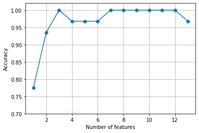
Sequential Backward Selection (SBS)

SBS is a greedy algorithm that starts with a complete set of features and removes the least important feature at each step, based on some metric, such as a decrease in the performance of the model or an increase in some measure of complexity.

The steps involved in SBS are as follows:

1. Start with the full set of features.

2. Train the model on the feature set and calculate a performance metric (such as classification accuracy or mean squared error).

3. Remove one feature from the feature set.

4. Train the model on the reduced feature set and calculate the performance metric.

5. If the performance metric has improved or has not changed significantly, keep the reduced feature set and go to step 3. Otherwise, stop and return the previous feature set.

6. Repeat steps 3-5 until the desired number of features is selected.

SBS can be useful in situations where the number of features is large and computational resources are limited. By iteratively removing features, SBS reduces the dimensionality of the feature space and improves the performance of the model by removing irrelevant or redundant features. SBS can be used with any type of machine learning algorithm that supports feature selection, such as linear regression, logistic regression, and support vector machines.

import numpy as np

from sklearn.base import clone
from itertools import combinations
from sklearn.metrics import accuracy_score
from sklearn.model_selection import train_test_split

class SBS():
  def __init__(self, estimator, k_features,
               scoring=accuracy_score,
               test_size=0.25, 
               random_state=1):
    self.scoring = scoring
    self.estimator = clone(estimator)
    self.k_features = k_features
    self.test_size = test_size
    self.random_state = random_state

  def fit(self, X, y):

    X_train, X_test, y_train, y_test = \
      train_test_split(X, y, test_size=self.test_size,
                       random_state=self.random_state)

    dim = X_train.shape[1]
    self.indices_ = tuple(range(dim))
    self.subsets_ = [self.indices_]
    score = self._calc_score(X_train, y_train,
                             X_test, y_test,
                             self.indices_)
    self.scores_ = [score]

    while dim > self.k_features:
      scores = []
      subsets = []

      for p in combinations(self.indices_, r=dim -1):
        score = self._calc_score(X_train, y_train,
                                 X_test, y_test, p)
        scores.append(score)
        subsets.append(p)

      best = np.argmax(scores)
      self.indices_ = subsets[best]
      self.subsets_.append(self.indices_)
      dim -= 1

      self.scores_.append(scores[best])

    self.k_score_ = self.scores_[-1]

    return self


  def transform(self, X):

    return X[:, self.indices_]


  def _calc_score(self, X_train, y_train, X_test, y_test, indices):

    self.estimator.fit(X_train[:, indices], y_train)
    y_pred = self.estimator.predict(X_test[:, indices])
    score = self.scoring(y_test, y_pred)

    return score

import matplotlib.pyplot as plt

from sklearn.neighbors import KNeighborsClassifier

knn = KNeighborsClassifier(n_neighbors=5)

sbs = SBS(knn, k_features=1)
sbs.fit(X_train_std, y_train)

k_feat = [len(k) for k in sbs.subsets_]

plt.plot(k_feat, sbs.scores_, marker='o')
plt.ylim([0.7, 1.02])
plt.ylabel('Accuracy')
plt.xlabel('Number of features')
plt.grid()
plt.show()

Assessing feature importance with random forests

from sklearn.ensemble import RandomForestClassifier

feat_labels = df_wine.columns[1:]

forest = RandomForestClassifier(n_estimators=500,
                                random_state=1)
forest.fit(X_train, y_train)
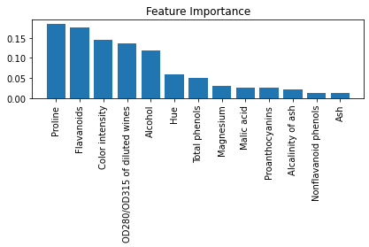
importances = forest.feature_importances_
indices = np.argsort(importances)[::-1]

for f in range(X_train.shape[1]):
  print("%2d: %-*s %f" % (f + 1, 30, 
                          feat_labels[indices[f]],
                          importances[indices[f]]))

plt.title('Feature Importance')
plt.bar(range(X_train.shape[1]),
        importances[indices],
        #importances,
        align='center')
plt.xticks(range(X_train.shape[1]),
            feat_labels[indices],
            rotation=90)
plt.xlim([-1, X_train.shape[1]])
plt.tight_layout()
plt.show()

Using the feature selection of Scikit-learn

from sklearn.feature_selection import SelectFromModel

sfm = SelectFromModel(forest, threshold=0.1,
                               prefit=True)
X_selected = sfm.transform(X_train)
print('Number of samples that meet this criterion:', 
      X_selected.shape[0])

for f in range(X_selected.shape[1]):
  print("%2d: %-*s %f" % (f + 1, 30,
                          feat_labels[indices[f]],
                          importances[indices[f]]))

Python Machine Learning 2nd Edition by Sebastian Raschka, Packt Publishing Ltd. 2017

Link: python-machine-learning-book-2nd-edition/ch04.ipynb at master · rasbt/python-machine-learning-book-2nd-edition (github.com)